

Predicting a Martian Apocalypse with Hypothesis Testing
Hypothesis Testing Explained in a Fun way

Predicting a Martian Apocalypse with Hypothesis Testing
We as humans make assumptions a lot of the time (knowingly or subconsciously). We tend to structure our understanding of the world around our own experiences, beliefs, interactions, etc. While we might believe things to be true, our truths are different. This begs the question of how to formalize this?
Statistical testing (AKA Hypothesis testing) is a procedure that can help to formalize the idea of testing out assumptions. You might have heard about this word from an introductory statistics class and gotten confused on things like the wording and why it works. For me personally, when I heard about hypothesis testing for the first time, I just remember being lost by all the mumbo jumbo terminology. This article aims to present a friendly introduction to hypothesis testing and build up a solid intuition for whatever endeavor you wish to pursue.
Storytime!
Before diving into hypothesis testing, it’s storytime! Grab a warm glass of milk (I personally am a Swiss Miss guy, but you do you!), a cozy blanket and get comfortable.
Imagine that we are in the year 2040 in New York City. Our technology has gotten so advanced and artificially intelligent beings are all around us. You grab your morning coffee at a Dunkin Donuts (though robot waiters prepped your coffee). You are about to take a subway to your office, but while you are waiting for it, you see a green figure standing idly. You haven’t seen such a figure, so walk towards it. The figure happened to resemble a human and the figure is about the same height as you. This figure definitely is not the Hulk, but you notice that the figure carries a Martian passport. You smile and worry. You are the first to see some extraterrestrial being, but are Martians trying to invade the Earth?
You reach our office and talk to Emily (your coworker) about what you saw. Emily is a bit surprised, but laughs off your observations.
“Are you sure that this ‘green being’ is a Martian? Maybe it’s just some green light reflection”, remarks Emily.
“Emily, this green being isn’t just a green light reflection. I distinctly saw this green figure with a passport saying the word ‘Martian’ in the pocket”, you explain.
“Do you really believe in Martians? Are you crazy?”, remarks Emily.
You respond, “When I saw this green figure carrying a Martian passport, something might be going wrong. Do you think we are headed towards a Martian apocalypse?”.
“Well, we know that aliens aren’t real. Even if you are being honest with me, I’m not sure how this one observation supports anything. I’m gonna need more proof”, said Emily.

How do we address this supposedly “crazy theory?”:
While this story might have been a bit strange, we need to help our character out. How can we test our crazy theory out? In a good experiment, we want to have a baseline to compare our results against. If we want to show that a Martian apocalypse might be happening, we might want to detect Martians for a good period of time. Let’s say for sake of simplicity that you use the same subway station for your daily commute to work. We will observe Martians over the course of 60 days. Each time we come to the subway station, we count up how many Martians we saw (luckily, our story describes how we know that we saw a Martian through the presence of the Martian passport).
We would have a table looking like this:

At first, we saw 1–2 Martians in the first week. 20–30 days in, we start to see more Martians (around 5–10 Martians). By the time the last 10 days are reached, we start to see 30+ Martians.
Now that we have the Martian counts for each day, you might say that “the Martian count went from 1–2 to 30+, so that is significant”, but another person might say “this increase in Martian count might not be significant. I’m not convinced”. This subjectivity of “what is considered significant?” is a major challenge of hypothesis testing. On top of that, we can’t just rely on gut instinct to say that an observation is significant vs. not-significant. Let’s be a bit more scientific!
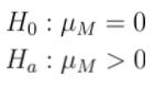
Instead of simply observing the trend in Martian counts over the 60 days, we could take the average of the Martian counts (ie: the mean) as we want to analyze if there is significant evidence to suggest a Martian apocalypse. If we let mu_{M} represent the mean Martian count, then we can formalize our problem as below:
Unpacking this notation, we have a few important points:
H0 represents the null hypothesis. You can think of this as the baseline. Recall that in our problem, we want to analyze if our mean Martian count is significantly different from what the mean would be in a world where “Martians don’t exist” (which would be 0). Our point of comparison is the part where Emily says that “we know that aliens aren’t real”.
Ha represents the alternative hypothesis. You can think of this as the assumption to test. In our problem, we had a suspicion that a Martian apocalypse was about to happen, so our assumption to test needs to suggest that the mean count of Martians is greater than 0.
Now that we have these components in place, we need to quantify where we draw the line between significant and non-significant. As you might suspect, we can pick this threshold ourselves, but we can identify if we fall above or below this threshold. We denote as the significance level. For sake of example, we will let alpha=0.05.
Carrying out the test:
Now that we have the nuts and bolts in place for mathematically testing if a Martian Apacolypse is happening, we need to actually carry out the test. First, we note that when collecting our data, we collected Martian counts over the time period of 60 days. Imagine repeating the process of collecting our Martian counts over 60 days and getting the mean Martian count for this process. We would form what’s called a sampling distribution of the mean. Don’t let this big phrase intimidate you. This distribution can be viewed as a histogram representing the counts of particular sample means (ie: how many samples/processes got mean of 30? 40? 50? etc). See the right side of the below image for a visual depiction:

It turns out that since our sample size of “60 days” is considered “large enough”, by the Central Limit Theorem, we can assume that the distribution of mean Martian counts is approximately normal.
Why is this nice?: With a normal distribution, we are able to easily calculate probabilities using the z-score (essentially a metric for standardization purposes).
Let’s assume that in our data, we find that the mean Martian count is 15 while the standard deviation of Martian counts (ie: average “spread”/variability) is 25. When we take a z-score, we use the below formula:
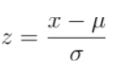
Where mu is the mean, sigma is the standard deviation. Calculating the z-score is called a standardization since we want to center the data point of interest x (relative to the mean) and “squishing the spread down to 1”. Essentially, we want to figure out “relative to the mean”, how far is x where the “unit” distance is . For example, if mu=3, x=7, sigma=2, then z=(7–3)/2=2 which means that “7” is 2 standard deviations to the right of 3 (because one unit = 2).
We will tweak this z-score formula a bit because when we calculate the standard deviation, we want to consider the sample size. When the sample size increases, the “spread” should ideally decrease because we have “more certainty”. We will instead use this z-score formula (don’t worry too much about the tweak we do with the standard deviation

Note that the s_{x} represents the sample standard deviation, x-bar is the sample mean and s_{x}/sqrt(n) represents the standard error (AKA, divide the standard deviation by the sample size).
From our given, x-bar = 15, s_{x} = 25 and n = 60. We want to find where our observation lies in the context where “Martians don’t exist. Therefore, mu = 0 since we are basing our observation relative to the null hypothesis.

Now that we have our z-score, in a context where the mean number of Martians is 0, our sample mean of 15 Martians is approximately 3.10 standard deviations to the right of 0. Now that we have an idea of where our sample mean lies relative to our null hypothesis, we need to check if our sample mean is significantly different from our null hypothesis sample mean.
Checking Significance:
Recall that in our alternative hypothesis, we stated that mu_{M} > 0. This signifies that we want to find the chance of getting a mean number of Martian counts that is more extreme than our sample mean of 15 Martians. To better understand this intuition, think back to the story. Emily wants to see proof that your observation of Martian counts is significant enough to lend itself to the possibility of a Martian apocalypse? If it is very unlikely that your mean Martian count will be higher than your sample mean of 15, then it signifies that your observation isn’t just a coincidence and we are more surprised. On the other hand, if there is a high likelihood that your mean Martian count will be higher than your observed sample mean, then your observation might be a “coincidence” and we are less surprised. It’s almost like comparing “it rained today” vs. “we had a big snowstorm” in California. Rain in California might be a reasonable expectation, but if somehow, it snowed in California, then you’re pretty surprised (what are the odds that it snows in California vs. it rains in California?). We can mimic this intuition by finding what’s called the p-value.
To find the p-value in this case, we want to find

as per our alternative hypothesis. Below is a snippet of our z-table.
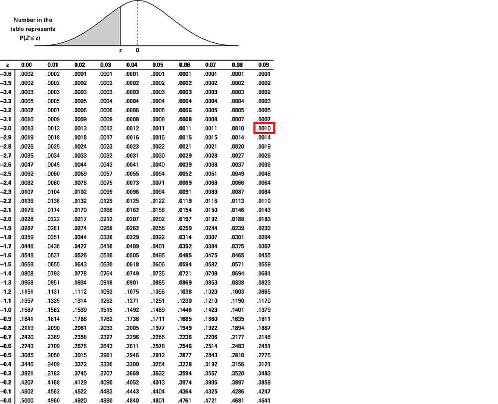
In our z-table, for each z-score z_{0} we find, we are able to find P(z < z_{0}). Since our z-table is symmetric, finding P(z > 3.09) is equivalent to finding P(z < -3.09) which is approximately 0.0010 (see the red box in Figure 9). Therefore, the probability of getting a mean Martian count more extreme than 15 is approximately 1/1000. Therefore, our sample mean of 15 Martians is quite surprising!
We initially assumed that our significance level is alpha = 0.05. This is our threshold for “significant” vs. “non-significant observations”. Earlier, we have established that being more surprised is good and that happens when the probability of getting an observation more extreme is very low. Thus, finding a p-value that falls below our significance level is grounds for saying that our observation is statistically significant. To contextualize in terms of our problem, the probability of getting a mean Martian count of above 15 is 1/1000 and since 0.0010 falls below our significance level of 0.05, our sample mean is statistically significant. Thus, we have evidence to conclude that a Martian apocalypse is possibly happening!
What happens now?:
You show your Martian count data and explain to Emily that your Martian counts are statistically significant through the hypothesis test we conduct (beyond a reasonable doubt though). Emily is flabbergasted! Emily plans on repeating your experiment and will present her findings to ensure you both are on the same page. Word starts to spread among your office and potentially, plans of action to protect us against the Martian apocalypse are put into place.

Conclusion:
Hopefully you found this article to be a fun way to introduce the concept of hypothesis testing without getting bogged down by the terminology. Now that you have the tools to mathematically test your assumptions, be curious. Go out there, explore, and keep learning something new each and every day! If there any questions or comments, feel free to post them.
This was a fun piece on something I had no knowledge about =)
Thanks Alex. Appreciate the kind words!